Log Storage and Analysis
Logs record key events in the system and contain crucial information such as the events' subject, time, location, and content. To meet the diverse needs of observability in operations, network security monitoring, and business analysis, enterprises might need to collect scattered logs for centralized storage, querying, and analysis to extract valuable content from the log data further.
In this scenario, Apache Doris provides a corresponding solution. With the characteristics of log scenarios in mind, Apache Doris added inverted-index and ultra-fast full-text search capabilities, optimizing write performance and storage space to the extreme. This allows users to build an open, high-performance, cost-effective, and unified log storage and analysis platform based on Apache Doris.
Focused on this solution, this chapter contains the following 3 sections:
Overall architecture: This section explains the core components and architecture of the log storage and analysis platform built on Apache Doris.
Features and advantages: This section explains the features and advantages of the log storage and analysis platform built on Apache Doris.
Operational guide: This section explains how to build a log storage and analysis platform based on Apache Doris.
Overall architecture
The following figure illustrates the architecture of the log storage and analysis platform built on Apache Doris:
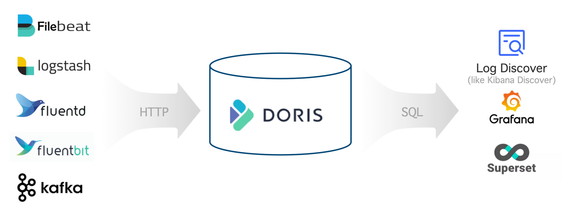
The architecture contains the following 3 parts:
Log collection and preprocessing: Various log collection tools can write log data into Apache Doris through HTTP APIs.
Log storage and analysis engine: Apache Doris provides high-performance, low-cost unified log storage, offering rich retrieval and analysis capabilities through SQL interfaces.
Log analysis and alert interface: Various log retrieval and analysis tools can query Apache Doris through standard SQL interfaces, providing users with a simple and user-friendly interface.
Features and advantages
The following figure illustrates the architecture of the log storage and analysis platform built on Apache Doris::
High throughput, low latency log writing: Supports stable writing of log data at the level of hundreds of TBs and GB/s per day, while maintaining latency within 1 second.
Cost-effective storage of massive log data: Supports petabyte-scale storage, saving 60% to 80% in storage costs compared to Elasticsearch, and further reducing storage costs by 50% by storing cold data in S3/HDFS.
High-performance log full-text search and analysis: Supports inverted indexes and full-text search, providing second-level response times for common log queries (keyword searches, trend analysis, etc.).
Open and user-friendly upstream and downstream ecosystem: Upstream integration with common log collection systems and data sources such as Logstash, Filebeat, Fluentbit, and Kafka through Stream Load's universal HTTP APIs, and downstream integration with various visual analytics UIs using standard MySQL protocol and syntax, such as observability platform Grafana, BI analytics Superset, and log retrieval Doris WebUI similar to Kibana.
Cost-effective performance
After Benchmark testing and production validation, the log storage and analysis platform built on Apache Doris has a 5 to 10 times cost-performance advantage over Elasticsearch. Apache Doris's performance benefits are mainly due to its globally leading high-performance storage and query engine, as well as specialized optimizations for log scenarios:
Improved write throughput: Elasticsearch's write performance bottleneck lies in CPU consumption for parsing data and building inverted indexes. In comparison, Apache Doris has optimized writes in two aspects: using SIMD and other CPU vector instructions to improve JSON data parsing speed and index-building performance and simplifying the inverted index structure for log scenarios by removing unnecessary data structures like forward indexes, effectively reducing index build complexity. With the same resources, Apache Doris's write performance is 3 to 5 times higher than Elasticsearch.
Reduced storage costs: Elasticsearch's storage bottleneck comes from multiple storage of forward, inverted, Docvalue columns, and lower compression ratios with general compression algorithms. Conversely, Apache Doris has optimized storage by eliminating forward indexes, reducing index data volume by 30%; adopting columnar storage and Zstandard compression algorithm, achieving compression ratios 5-10 times higher than Elasticsearch's 1.5 times; with low access frequency of cold data in log data, Apache Doris's cold-hot tiering feature can automatically store logs older than defined period in lower-cost object storage, reducing cold data storage costs by over 70%. For the same original data, Select
Strong analytical capabilities
Apache Doris supports standard SQL and is compatible with MySQL protocol and syntax. Therefore, log systems built on Apache Doris can use SQL for log analysis, giving the following advantages to log systems:
Easy to use: Engineers and data analysts are very familiar with SQL, their expertise can be reused, no need to learn new technology stacks to quickly get started.
Rich ecosystem: The MySQL ecosystem is the most widely used language in the database field, seamlessly integrating with and applying to the MySQL ecosystem. Doris can leverage MySQL command line and various GUI tools, BI tools, and other big data ecosystem tools for more complex and diverse data processing and analysis needs.
Strong analytical capabilities: SQL has become the de facto standard for database and big data analysis, with powerful expressive capabilities and functions supporting retrieval, aggregation, multi-table JOIN, subqueries, UDFs, logical views, materialized views, and various data analysis capabilities.
Flexible Schema
Here is a typical example of a semi-structured log in JSON format. The top-level fields are some fixed fields, such as timestamp, source, node, component, level, clientRequestID, message, and properties, which are present in every log entry. The nested fields of the properties , such as properties.size and properties.format are more dynamic, and the fields of each log may vary.
{
"timestamp": "2014-03-08T00:50:03.8432810Z",
"source": "ADOPTIONCUSTOMERS81",
"node": "Engine000000000405",
"level": "Information",
"component": "DOWNLOADER",
"clientRequestId": "671db15d-abad-94f6-dd93-b3a2e6000672",
"message": "Downloading file path: benchmark/2014/ADOPTIONCUSTOMERS81_94_0.parquet.gz",
"properties": {
"size": 1495636750,
"format": "parquet",
"rowCount": 855138,
"downloadDuration": "00:01:58.3520561"
}
}
Apache Doris provides several aspects of support for Flexible Schema log data:
For minor changes to top-level fields, Light Schema Change can be used to add or remove columns and to add or remove indexes, enabling schema changes to be completed in seconds. When planning a log platform, users only need to consider which fields need to be indexed.
For extension fields similar to properties, the native semi-structured data type
VARIANTis provided, which can write any JSON data, automatically recognize field names and types in JSON, and automatically split frequently occurring fields for columnar storage for subsequent analysis. Additionally,VARIANTcan create inverted indexes to accelerate internal field queries and retrievals.
Compared to Elasticsearch's Dynamic Mapping, Apache Doris's Flexible Schema has the following advantages:
Allows a field to have multiple types,
VARIANTautomatically handles conflicts and type promotion for fields, better adapting to iterative changes in log data.VARIANTautomatically merges infrequently occurring fields into a column store to avoid performance issues caused by excessive fields, metadata, or columns.Not only can columns be dynamically added, but they can also be dynamically deleted, and indexes can be dynamically added or removed, eliminating the need to index all fields at the beginning like Elasticsearch, reducing unnecessary costs.
Operational guide
Step 1: Estimate resources
Before deploying the cluster, you need to estimate the hardware resources required for the servers. Follow the steps below:
- Estimate the resources for data writing by the following calculation formulas:
Daily data increment / 86400 s = Average write throughput
Average write throughput * Ratio of the peak write throughput to the average write throughput = Peak write throughput
Peak write throughput / Write throughput of a single-core CPU = Number of CPU cores for the peak write throughput
Estimate the resources for data storage by the calculation formula: Daily data increment / Data compression ratio * Number of data copies * Data storage duration = Data storage space.
Estimate the resources for data querying. The resources for data querying depend on the query volume and complexity. It is recommended to reserve 50% of CPU resources for data query initially and then adjust according to the actual test results.
Integrate the calculation results as follows:
Divide the number of CPU cores calculated in Step 1 and Step 3 by the number of CPU cores of a BE server, and you can get the number of BE servers.
Based on the number of BE servers and the calculation result of Step 2, estimate the storage space required for each BE server.
Allocate the storage space required for each BE server to 4 to 12 data disks, and you can get the storage capacity required for a single data disk.
For example, suppose that the daily data increment is 100 TB, the data compression ratio is 7, the number of data copies is 1, the storage duration of hot data is 3 days, the storage duration of cold data is 30 days, the ratio of the peak write throughput to the average write throughput is 200%, the write throughput of a single-core CUP is 10 MB/s, and 50% of CPU resources are reserved for data querying, one can estimate that:
3 FE servers are required, each configured with a 16-core CPU, 64 GB memory, and an 1100 GB SSD disk.
15 BE servers are required, each configured with a 32-core CPU, 256 GB memory, and 8 500 GB SSD disks.
S3:430 TB
Refer to the following table to learn about the values of indicators in the example above and how they are calculated.
| Indicator (Unit) | Value | Description |
|---|---|---|
| Daily data increment (TB) | 100 | Specify the value according to your actual needs. |
| Data compression ratio | 7 | Specify the value according to your actual needs, which is often between 5 to 10. Note that the data contains index data. |
| Number of data copies | 1 | Specify the value according to your actual needs, which can be 1, 2, or 3. The default value is 1. |
| Storage duration of hot data (day) | 3 | Specify the value according to your actual needs. |
| Storage duration of cold data (day) | 30 | Specify the value according to your actual needs. |
| Data storage duration | 33 | Calculation formula: Storage duration of hot data + Storage duration of cold data |
| Estimated storage space for hot data (TB) | 42.9 | Calculation formula: Daily data increment / Data compression ratios * Number of data copies * Storage duration of hot data |
| Estimated storage space for cold data (TB) | 428.6 | Calculation formula: Daily data increment / Data compression ratios * Number of data copies * Storage duration of cold data |
| Ratio of the peak write throughput to the average write throughput | 200% | Specify the value according to your actual needs. The default value is 200%. |
| Number of CPU cores of a BE server | 32 | Specify the value according to your actual needs. The default value is 32. |
| Average write throughput (MB/s) | 1214 | Calculation formula: Daily data increment / 86400 s |
| Peak write throughput (MB/s) | 2427 | Calculation formula: Average write throughput * Ratio of the peak write throughput to the average write throughput |
| Number of CPU cores for the peak write throughput | 242.7 | Calculation formula: Peak write throughput / Write throughput of a single-core CPU |
| Percent of CPU resources reserved for data querying | 50% | Specify the value according to your actual needs. The default value is 50%. |
| Estimated number of BE servers | 15.2 | Calculation formula: Number of CPU cores for the peak write throughput / Number of CPU cores of a BE server /(1 - Percent of CPU resources reserved for data querying) |
| Rounded number of BE servers | 15 | Calculation formula: MAX (Number of data copies, Estimated number of BE servers) |
| Estimated data storage space for each BE server (TB) | 4.03 | Calculation formula: Estimated storage space for hot data / Estimated number of BE servers /(1 - 30%), where 30% represents the percent of reserved storage space. It is recommended to mount 4 to 12 data disks on each BE server to enhance I/O capabilities. |
Step 2: Deploy the cluster
After estimating the resources, you need to deploy the cluster. It is recommended to deploy in both physical and virtual environments manually. For manual deployment, refer to Manual Deployment.
Alternatively, it is recommended to use VeloDB Manager provided by VeloDB Enterprise to deploy the cluster, reducing overall deployment costs. For more information about the VeloDB Manager, please refer to the following documents:
Step 3: Optimize FE and BE configurations
After completing the cluster deployment, it is necessary to optimize the configuration parameters for both the front-end and back-end separately, so as to better suit the scenario of log storage and analysis.
Optimize FE configurations
You can find FE configuration fields in fe/conf/fe.conf. Refer to the following table to optimize FE configurations.
| Configuration fields to be optimized | Description |
|---|---|
max_running_txn_num_per_db = 10000 | Increase the parameter value to adapt to high-concurrency import transactions. |
streaming_label_keep_max_second = 3600``label_keep_max_second = 7200 | Increase the retention time to handle high-frequency import transactions with high memory usage. |
enable_round_robin_create_tablet = true | When creating Tablets, use a Round Robin strategy to distribute evenly. |
tablet_rebalancer_type = partition | When balancing Tablets, use a strategy to evenly distribute within each partition. |
enable_single_replica_load = true | Enable single-replica import, where multiple replicas only need to build an index once to reduce CPU consumption. |
autobucket_min_buckets = 10 | Increase the minimum number of automatically bucketed buckets from 1 to 10 to avoid insufficient buckets when the log volume increases. |
max_backend_heartbeat_failure_tolerance_count = 10 | In log scenarios, the BE server may experience high pressure, leading to short-term timeouts, so increase the tolerance count from 1 to 10. |
For more information, refer to FE Configuration.
Optimize BE configurations
You can find BE configuration fields in be/conf/be.conf. Refer to the following table to optimize BE configurations.
| Module | Configuration fields to be optimized | Description |
|---|---|---|
| Storage | storage_root_path = /path/to/dir1;/path/to/dir2;...;/path/to/dir12 | Configure the storage path for hot data on disk directories. |
| - | enable_file_cache = true | Enable file caching. |
| - | file_cache_path = [{"path": "/mnt/datadisk0/file_cache", "total_size":53687091200, "query_limit": "10737418240"},{"path": "/mnt/datadisk1/file_cache", "total_size":53687091200,"query_limit": "10737418240"}] | Configure the cache path and related settings for cold data with the following specific configurations:path: cache pathtotal_size: total size of the cache path in bytes, where 53687091200 bytes equals 50 GBquery_limit: maximum amount of data that can be queried from the cache path in one query in bytes, where 10737418240 bytes equals 10 GB |
| Write | write_buffer_size = 1073741824 | Increase the file size of the write buffer to reduce small files and random I/O operations, improving performance. |
| - | max_tablet_version_num = 20000 | In coordination with the time_series compaction strategy for table creation, allow more versions to remain temporarily unmerged |
| - | enable_single_replica_load = true | Enable single replica import to reduce CPU consumption, consistent with FE configuration. |
| Compaction | max_cumu_compaction_threads = 8 | Set to CPU core count / 4, indicating that 1/4 of CPU resources are used for writing, 1/4 for background compaction, and 2/1 for queries and other operations. |
| - | inverted_index_compaction_enable = true | Enable inverted index compaction to reduce CPU consumption during compaction. |
| - | enable_segcompaction = false enable_ordered_data_compaction = false | Disable two compaction features that are unnecessary for log scenarios. |
| Cache | disable_storage_page_cache = true inverted_index_searcher_cache_limit = 30% | Due to the large volume of log data and limited caching effect, switch from data caching to index caching. |
| - | inverted_index_cache_stale_sweep_time_sec = 3600 index_cache_entry_stay_time_after_lookup_s = 3600 | Maintain index caching in memory for up to 1 hour. |
| - | enable_inverted_index_cache_on_cooldown = trueenable_write_index_searcher_cache = false | Enable automatic caching of cold data storage during index uploading. |
| - | tablet_schema_cache_recycle_interval = 3600 segment_cache_capacity = 20000 | Reduce memory usage by other caches. |
| Thread | pipeline_executor_size = 24 doris_scanner_thread_pool_thread_num = 48 | Configure computing threads and I/O threads for a 32-core CPU in proportion to core count. |
| - | scan_thread_nice_value = 5 | Lower the priority of query I/O threads to ensure writing performance and timeliness. |
| Other | string_type_length_soft_limit_bytes = 10485760 | Increase the length limit of string-type data to 10 MB. |
| - | trash_file_expire_time_sec = 300 path_gc_check_interval_second = 900 path_scan_interval_second = 900 | Accelerate the recycling of trash files. |
For more information, refer to BE Configuration.
Step 4: Create tables
Due to the distinct characteristics of both writing and querying log data, it is recommended to configure tables with targeted settings to enhance performance.
Configure data partitioning and bucketing
For data partitioning:
Enable range partitioning with dynamic partitions managed automatically by day.
Use a field in the DATETIME type as the key for accelerated retrieval of the latest N log entries.
For data bucketing:
Configure the number of buckets to be roughly three times the total number of disks in the cluster.
Use the Random strategy to optimize batch writing efficiency when paired with single tablet imports.
For more information, refer to Data Partitioning.
Configure compaction fileds
Configure compaction fields as follows:
Use the time_series strategy to reduce write amplification, which is crucial for high-throughput log writes.
Use single-replica compaction to minimize the overhead of multi-replica compaction.
Configure index fields
Configuring index fields as follows:
Create indexes for fields that are frequently queried.
For fields that require full-text search, specify the parser field as unicode, which satisfies most requirements. If there is a need to support phrase queries, set the support_phrase field to true; if not needed, set it to false to reduce storage space.
Configure storage policies
Configure storage policies as follows:
For storage of hot data, if using cloud storage, configure the number of data copies as 1; if using physical disks, configure the number of data copies as at least 2.
Configure the storage location for log_s3 and set the log_policy_3day policy, where the data is cooled and moved to the specified storage location of log_s3 after 3 days. Refer to the code below.
CREATE DATABASE log_db;
USE log_db;

CREATE RESOURCE "log_s3"
PROPERTIES
(
    "type" = "s3",
    "s3.endpoint" = "your_endpoint_url",
    "s3.region" = "your_region",
    "s3.bucket" = "your_bucket",
    "s3.root.path" = "your_path",
    "s3.access_key" = "your_ak",
    "s3.secret_key" = "your_sk"
);

CREATE STORAGE POLICY log_policy_3day
PROPERTIES(
    "storage_resource" = "log_s3",
    "cooldown_ttl" = "259200"
);

CREATE TABLE log_table
(
  `ts` DATETIME,
  `host` TEXT,
  `path` TEXT,
  `message` TEXT,
  INDEX idx_host (`host`) USING INVERTED,
  INDEX idx_path (`path`) USING INVERTED,
  INDEX idx_message (`message`) USING INVERTED PROPERTIES("parser" = "unicode", "support_phrase" = "true")
)
ENGINE = OLAP
DUPLICATE KEY(`ts`)
PARTITION BY RANGE(`ts`) ()
DISTRIBUTED BY RANDOM BUCKETS 250
PROPERTIES (
"dynamic_partition.enable" = "true",
"dynamic_partition.create_history_partition" = "true",
"dynamic_partition.time_unit" = "DAY",
"dynamic_partition.start" = "-30",
"dynamic_partition.end" = "1",
"dynamic_partition.prefix" = "p",
"dynamic_partition.buckets" = "250",
"dynamic_partition.replication_num" = "1", -- unneccessary for the compute-storage coupled mode
"replication_num" = "1" -- unneccessary for the compute-storage coupled mode
"enable_single_replica_compaction" = "true", -- unneccessary for the compute-storage coupled mode
"storage_policy" = "log_policy_3day", -- unneccessary for the compute-storage coupled mode
"compaction_policy" = "time_series"
);
Step 5: Collect logs
After completing table creation, you can proceed with log collection.
Apache Doris provides open and versatile Stream HTTP APIs, through which you can connect with popular log collectors such as Logstash, Filebeat, Kafka, and others to carry out log collection work. This section explains how to integrate these log collectors using the Stream HTTP APIs.
Integrating Logstash
Follow these steps:
Download and install the Logstash Doris Output plugin. You can choose one of the following two methods:
Click to download and install.
Compile from the source code and run the following command to install:
./bin/logstash-plugin install logstash-output-doris-1.0.0.gem
Configure Logstash. Specify the following fields:
logstash.yml: Used to configure Logstash batch processing log sizes and timings for improved data writing performance.
pipeline.batch.size: 1000000
pipeline.batch.delay: 10000logstash_demo.conf: Used to configure the specific input path of the collected logs and the settings for output to Apache Doris.
input {
file {
path => "/path/to/your/log"
}
}
<br />output {
doris {
http_hosts => \[ "<http://fehost1:http_port>", "<http://fehost2:http_port>", "<http://fehost3:http_port"\>]
user => "your_username"
password => "your_password"
db => "your_db"
table => "your_table"
\# doris stream load http headers
headers => {
"format" => "json"
"read_json_by_line" => "true"
"load_to_single_tablet" => "true"
}
\# field mapping: doris fileld name => logstash field name
\# %{} to get a logstash field, \[\] for nested field such as \[host\]\[name\] for host.name
mapping => {
"ts" => "%{@timestamp}"
"host" => "%{\[host\]\[name\]}"
"path" => "%{\[log\]\[file\]\[path\]}"
"message" => "%{message}"
}
log_request => true
log_speed_interval => 10
}
}
Run Logstash according to the command below, collect logs, and output to Apache Doris.
./bin/logstash -f logstash_demo.conf
For more information about the Logstash Doris Output plugin, see Logstash Doris Output Plugin.
Integrating Filebeat
Follow these steps:
Obtain the Filebeat binary file that supports output to Apache Doris. You can click to download or compile it from the Apache Doris source code.
Configure Filebeat. Specify the filebeat_demo.yml field that is used to configure the specific input path of the collected logs and the settings for output to Apache Doris.
# input
filebeat.inputs:
- type: log
enabled: true
paths:
    - /path/to/your/log
multiline:
    type: pattern
    pattern: '^[0-9]{4}-[0-9]{2}-[0-9]{2} [0-9]{2}:[0-9]{2}:[0-9]{2}'
    negate: true
    match: after
    skip_newline: true

processors:
- script:
    lang: javascript
    source: >
        function process(event) {
            var msg = event.Get("message");
            msg = msg.replace(/\t/g, "  ");
            event.Put("message", msg);
        }
- dissect:
    # 2024-06-08 18:26:25,481 INFO (report-thread|199) [ReportHandler.cpuReport():617] begin to handle
    tokenizer: "%{day} %{time} %{log_level} (%{thread}) [%{position}] %{content}"
    target_prefix: ""
    ignore_failure: true
    overwrite_keys: true

# queue and batch
queue.mem:
events: 1000000
flush.min_events: 100000
flush.timeout: 10s

# output
output.doris:
fenodes: [ "http://fehost1:http_port", "http://fehost2:http_port", "http://fehost3:http_port" ]
user: "your_username"
password: "your_password"
database: "your_db"
table: "your_table"
# output string format
codec_format_string: '{"ts": "%{[day]} %{[time]}", "host": "%{[agent][hostname]}", "path": "%{[log][file][path]}", "message": "%{[message]}"}'
headers:
    format: "json"
    read_json_by_line: "true"
    load_to_single_tablet: "true"
Run Filebeat according to the command below, collect logs, and output to Apache Doris.
chmod +x filebeat-doris-1.0.0
./filebeat-doris-1.0.0 -c filebeat_demo.yml
For more information about Filebeat, refer to Beats Doris Output Plugin.
Integrating Kafka
Write JSON formatted logs to Kafka's message queue, create a Kafka Routine Load, and allow Apache Doris to actively pull data from Kafka.
You can refer to the example below, where property.\* represents Librdkafka client-related configurations and needs to be adjusted according to the actual Kafka cluster situation.
CREATE ROUTINE LOAD load_log_kafka ON log_db.log_table
COLUMNS(ts, clientip, request, status, size)
PROPERTIES (
"max_batch_interval" = "10",
"max_batch_rows" = "1000000",
"max_batch_size" = "109715200",
"load_to_single_tablet" = "true",
"timeout" = "600",
"strict_mode" = "false",
"format" = "json"
)
FROM KAFKA (
"kafka_broker_list" = "host:port",
"kafka_topic" = "log_\_topic_",
"property.group.id" = "your_group_id",
"property.security.protocol"="SASL_PLAINTEXT",
"property.sasl.mechanism"="GSSAPI",
"property.sasl.kerberos.service.name"="kafka",
"property.sasl.kerberos.keytab"="/path/to/xxx.keytab",
"property.sasl.kerberos.principal"="<xxx@yyy.com>"
);
<br />SHOW ROUTINE LOAD;
For more information about Kafka, see Routine Load。
Using customized programs to collect logs
In addition to integrating common log collectors, you can also customize programs to import log data into Apache Doris using the Stream Load HTTP API. Refer to the following code:
curl \\
\--location-trusted \\
\-u username:password \\
\-H "format:json" \\
\-H "read_json_by_line:true" \\
\-H "load_to_single_tablet:true" \\
\-H "timeout:600" \\
\-T logfile.json \\
http://fe_host:fe_http_port/api/log_db/log_table/\_stream_load
When using custom programs, pay attention to the following key points:
Use Basic Auth for HTTP authentication, calculate using the command echo -n 'username:password' | base64.
Set HTTP header "format:json" to specify the data format as JSON.
Set HTTP header "read_json_by_line:true" to specify one JSON per line.
Set HTTP header "load_to_single_tablet:true" to import data into one bucket at a time to reduce small file imports.
It is recommended to write batches whose sizes are between 100MB to 1GB on the client side. For Apache Doris version 2.1 and higher, you need to reduce batch sizes on the client side through the Group Commit function.
Step 6: Query and analyze logs
Query logs
Apache Doris supports standard SQL, so you can connect to the cluster through MySQL client or JDBC to execute SQL for log queries.
mysql -h fe_host -P fe_mysql_port -u your_username -Dyour_db_name
Here are 5 common SQL query commands for reference:
- View the latest 10 log entries
SELECT \* FROM your_table_name ORDER BY ts DESC LIMIT 10;
- Query the latest 10 log entries with the host as 8.8.8.8
SELECT \* FROM your_table_name WHERE host = '8.8.8.8' ORDER BY ts DESC LIMIT 10;
- Retrieve the latest 10 log entries with error or 404 in the request field. In the command below, MATCH_ANY is a full-text search SQL syntax used by Apache Doris for matching any keyword in the fields.
SELECT \* FROM your_table_name WHERE message **MATCH_ANY** 'error 404'
ORDER BY ts DESC LIMIT 10;
- Retrieve the latest 10 log entries with image and faq in the request field. In the command below, MATCH_ALL is a full-text search SQL syntax used by Apache Doris for matching all keywords in the fields.
SELECT \* FROM your_table_name WHERE message **MATCH_ALL** 'image faq'
ORDER BY ts DESC LIMIT 10;
- Retrieve the latest 10 entries with image and faq in the request field. In the following command, MATCH_PHRASE is a full-text search SQL syntax used by Apache Doris for matching all keywords in the fields and requiring consistent order. In the example below, a image faq b can match, but a faq image b cannot match because the order of image and faq does not match the syntax.
SELECT \* FROM your_table_name WHERE message **MATCH_PHRASE** 'image faq'
ORDER BY ts DESC LIMIT 10;
Analyze logs visually
VeloDB Enterprise Core, built on Apache Doris, provides a data development platform called VeloDB Enterprise WebUI ("WebUI"), featuring a Kibana Discover-like log retrieval and analysis interface for intuitive and easy exploratory log analysis interaction as shown in the image below:
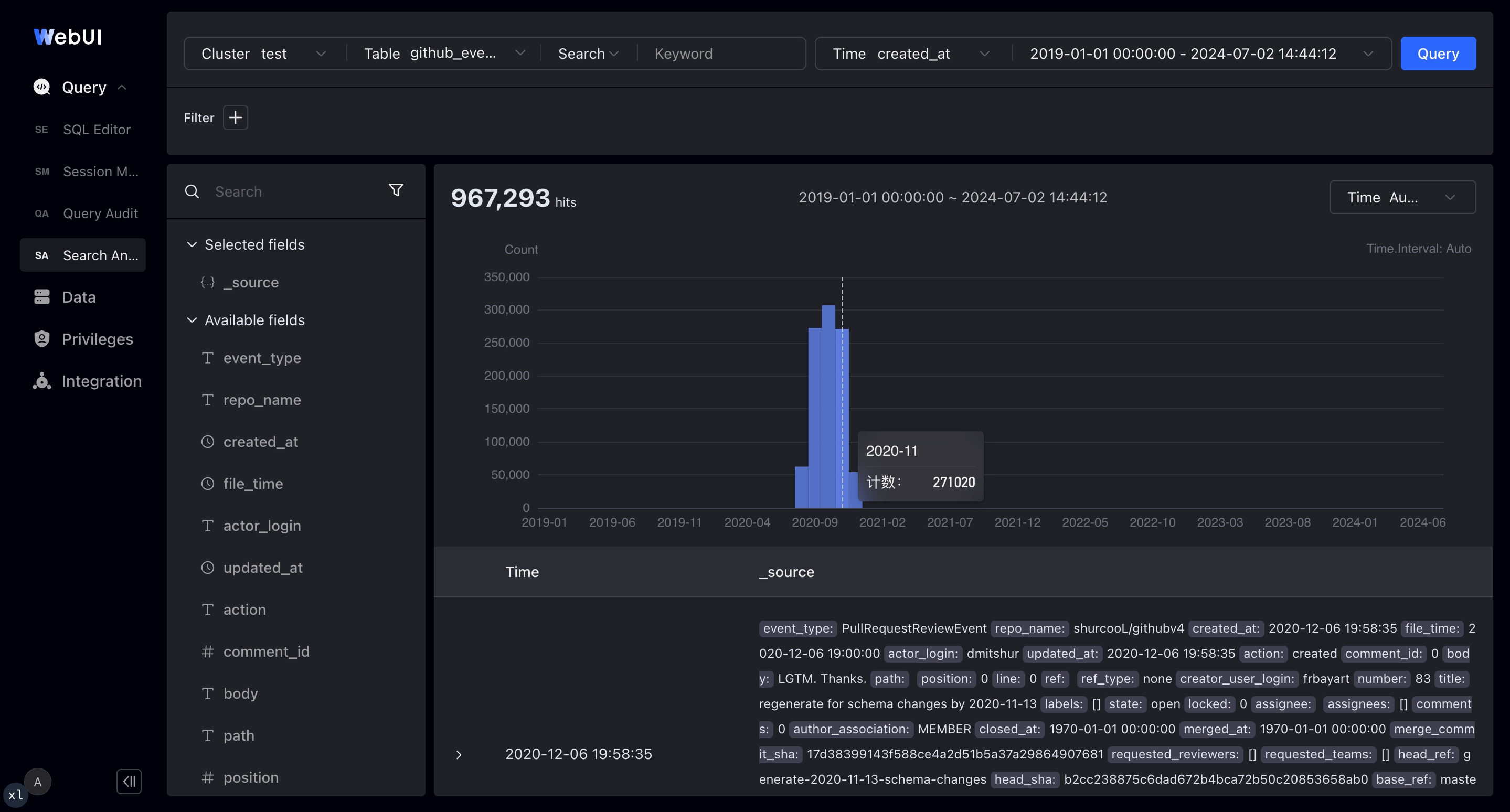
On this interface, WebUI supports the following operations:
Support for full-text search and SQL modes
Support for selecting query log timeframes with time boxes and histograms
Display of detailed log information, expandable into JSON or tables
Interactive clicking to add and remove filter conditions in the log data context
Display of top field values in search results for finding anomalies and further drilling down for analysis
You can click to download VeloDB Enterprise Core and install it to use WebUI. For more information about the main functions and how to use WebUI, see WebUI.